
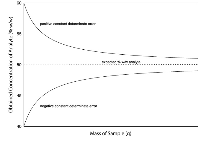
The magnitude of a constant determinate error is the same for all samples and is more significant when analyzing smaller samples. Analyzing samples of different sizes, therefore, allows us to detect a constant determinate error. For example, consider a quantitative analysis in which we separate the analyte from its matrix and determine its mass. Let’s assume the sample is 50.0% w/w analyte, which means the expected amount of analyte in a 0.100 g sample is 0.050 g. If the analysis has a positive constant determinate error of 0.010 g, then analyzing the sample gives 0.060 g of analyte and we report the analyte’ concentration as 60.0% w/w. If we increase the sample’s size to 0.800 g, then we find that the sample contains 0.410 g of analyte (0.400 g from the sample and 0.010 g from the constant determinate error) and report analyte’s concentration as 51.2% w/w, a result much closer to its true value of 50.0% w/w. If we plot the analyte’s concentration as a function of the amount of sample taken, then an upward or downward trend, as shown here, provides evidence of a constant determinate error.